

本博客为 kaggle 房价预测 的代码和实验报告,并融合自己的心得。
本实验在 23 年做过一次。25年 必修课程要求 写报告而有了些新的感悟。
实验报告格式根据 智能算法综合实践 课程要求。
比赛界面:房价预测
我的开源 jupyter notebook :线性回归 ,MLP 和多种优化
一、前言 #
我想将 jupyter notebook 的输出汇总到本报告之中,但转化无法避免的导致排版略显杂乱,请理解。
本实验报告很大一部分是由 jupyter notebook 转化 md 而得到的:
jupyter nbconvert name.ipynb --to markdown
而 word 版本使用了:
pandoc name.md -o output.docx
网络搭建部分参考了李沐老师的波士顿房价预测实例。
二、实验目的 #
在 Kaggle 房价预测竞赛中构建模型并优化性能。
掌握数据预处理、特征工程及回归任务建模方法。
熟悉 PyTorch 的基本操作,包括数据处理、模型训练与评估。
其中关于 PyTorch 操作,借由本次实验我进行了一定程度的总结,见我的博客:pytorch 总结
三、实验原理与实验步骤 #
线性回归 #
显然该问题是一个回归问题,先试一下最简单的线性回归。
线性回归在现在的 pytorch 中框架非常简单,几乎一个 nn.linear() 就能解决。
对数据进行一定的操作:
-
对 features 进行归一化,这几乎在任何线性回归任务中都是必须的。
-
该题最终检测的是 RMSE,但经过我的测试,loss 用 nn.MSELoss() 仍是最佳的。
-
因此为了使检测数据更加直观,要手写一个 RMSE 用于检测输出。
RMSE 是 MSE 开方后的值,它的最优点与 MSE 一致,只是数值上有非线性变化(平方根)。
-
该题的输入样式很多,包括 bool,int,float 等,要将其统一到 tensor 中。
-
将 bool 值进行热编码。
为了检验拟合情况,使用了 K 折交叉检验(这为我判断是否过拟合起到了很大的帮助)
此外,为了直观观察 loss 下降,我也做了适配 RMSE 的绘图。
此方案提交后的结果为 :0.149,排名大致为 2000 / 3700
MLP 与优化 #
在线性回归之后,很正常的思路是将模型扩大,即使用 MLP 进行学习。
当然,使用 MLP 就代表要使用 cuda 加速,需要修改 to(device) 。
但在仅修改 MLP 后,最后效果却反而不如线性回归,原因有以下几点:
- 出现了严重的过拟合,MLP 神经元较多导致学习了很多不相干特征的。
- 实际损失函数 MSE 在不同房价基础上的表现有所差异。
对于第二点,我尝试过用 RMSE 做损失函数,但效果并不好。
为了修改 MSE 的表现需要将 label 进行归一化,并在实际预测时进行反归一化。
对于第一点,修改分成的两部分:
- 适当缩小 MLP 的神经元数量、dropout 设置为 0.5、加入 L2 正则化。
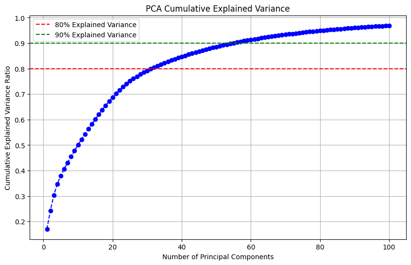
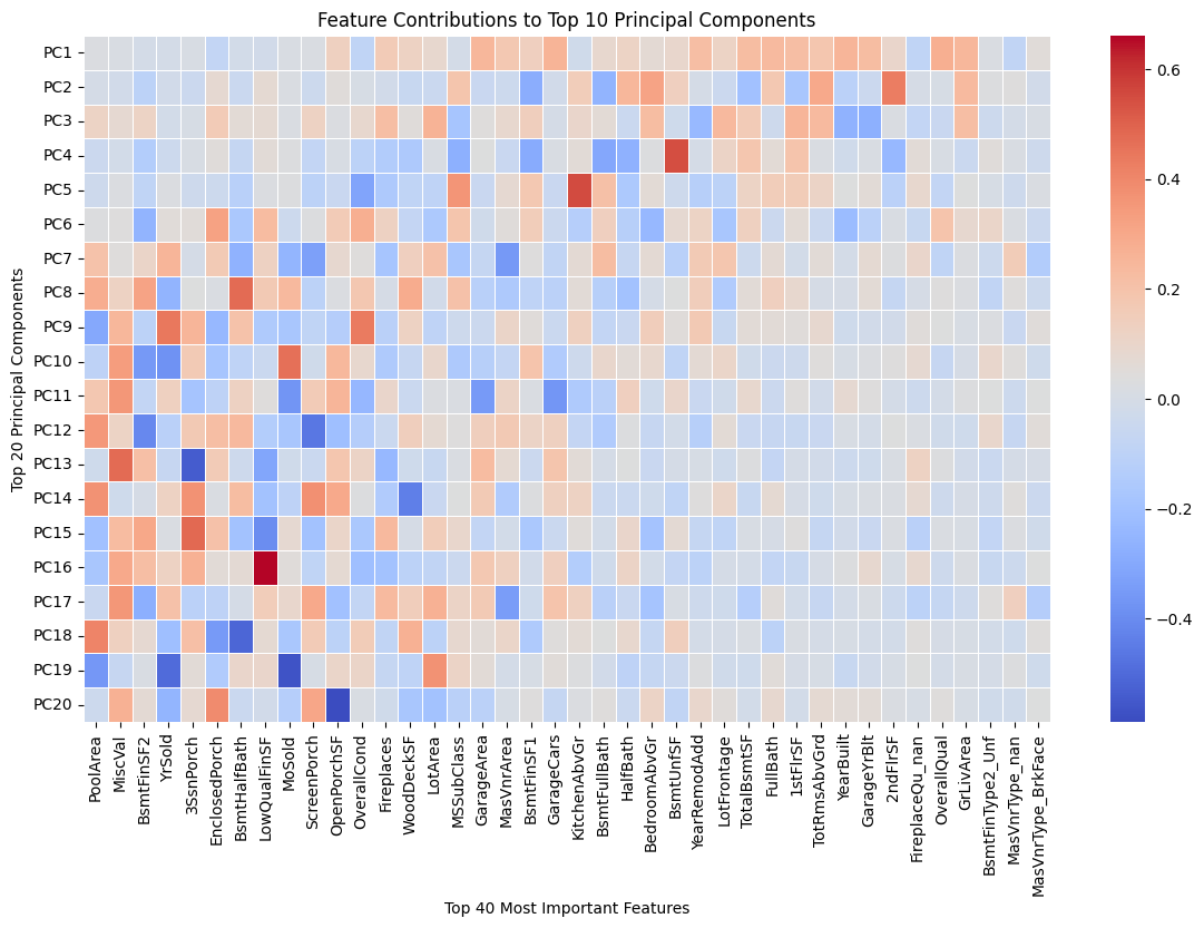
- 对输入进行主成分分析(具体可视化在 MLP 一节的特征工程小节),选取了前 100 个主成分(累计贡献 98%)。
当然,修改过后还有一定的过拟合现象,但并不严重。
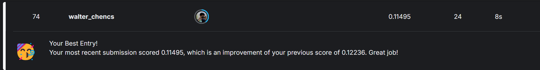
此方案提交后的结果为 :0.122,排名大致为 250 / 3700

如果进行仔细的调参,还有一定的提升空间。
特征工程 #
在参考排行榜头部 notebook 后,我发现此题最重要的部分是特征工程。
即使上一部分中,我使用了主成分分析,但仍远远不如直接从特征出发。
参考大量他人文档,引用了高分公开测试集,经过一定的参数调整后,得到结果如下。
但我个人认为,这种针对数据集的调整的泛用性不一定强。因此在大部分实际工作中,并不具有普遍性。
四、具体实验 #
简单线性回归 #
首先检查 input #
特别是训练集和测试集的 shape
# This Python 3 environment comes with many helpful analytics libraries installed
# It is defined by the kaggle/python Docker image: https://github.com/kaggle/docker-python
# For example, here's several helpful packages to load

import numpy as np # linear algebra
import pandas as pd # data processing, CSV file I/O (e.g. pd.read_csv)

# Input data files are available in the read-only "../input/" directory
# For example, running this (by clicking run or pressing Shift+Enter) will list all files under the input directory

import os
for dirname, _, filenames in os.walk('/kaggle/input'):
    for filename in filenames:
        print(os.path.join(dirname, filename))

# You can write up to 20GB to the current directory (/kaggle/working/) that gets preserved as output when you create a version using "Save & Run All"
# You can also write temporary files to /kaggle/temp/, but they won't be saved outside of the current session
/kaggle/input/house-prices-advanced-regression-techniques/sample_submission.csv
/kaggle/input/house-prices-advanced-regression-techniques/data_description.txt
/kaggle/input/house-prices-advanced-regression-techniques/train.csv
/kaggle/input/house-prices-advanced-regression-techniques/test.csv
train_data = pd.read_csv("/kaggle/input/house-prices-advanced-regression-techniques/train.csv")
test_data = pd.read_csv("/kaggle/input/house-prices-advanced-regression-techniques/test.csv")

print("Train Data Shape:", train_data.shape)
print("Test Data Shape:", test_data.shape)
Train Data Shape: (1460, 81)
Test Data Shape: (1459, 80)
进行特征工程 #
将 input 进行 transform
# 检查列名
print(train_data.iloc[0, :])
print("-------------")
print(test_data.iloc[0, :])
# 其中 test_data 没有最后的 SalePrice
Id                    1
MSSubClass           60
MSZoning             RL
LotFrontage        65.0
LotArea            8450
                  ...
MoSold                2
YrSold             2008
SaleType             WD
SaleCondition    Normal
SalePrice        208500
Name: 0, Length: 81, dtype: object
-------------
Id                 1461
MSSubClass           20
MSZoning             RH
LotFrontage        80.0
LotArea           11622
                  ...
MiscVal               0
MoSold                6
YrSold             2010
SaleType             WD
SaleCondition    Normal
Name: 0, Length: 80, dtype: object
显然 id 这一列对数据预测没有实际意义
对特征进行整合,并准备进行特征工程
features = pd.concat((train_data.iloc[:, 1:-1], test_data.iloc[:, 1:]))
print(features.shape)
print("--------")
print(features.iloc[0, :])
(2919, 79)
--------
MSSubClass           60
MSZoning             RL
LotFrontage        65.0
LotArea            8450
Street             Pave
                  ...
MiscVal               0
MoSold                2
YrSold             2008
SaleType             WD
SaleCondition    Normal
Name: 0, Length: 79, dtype: object
将数组进行归一化,如公式所示 $$ (x - \mu) / \sigma$$
# numeric_features 是特征中非对象类型(即整数与浮点数)的 index
numeric_features = features.dtypes[features.dtypes != 'object'].index
features[numeric_features] = features[numeric_features].apply(
    lambda x: (x - x.mean()) / (x.std()))
# 在标准化数据之后,所有均值消失。因此我们可以将缺失值设置为 0
features[numeric_features] = features[numeric_features].fillna(0)
# 接下来处理布尔值。dummy_na 表示是否单独提出 nan
在新版本下,get_dummies 会转化为 uint8
但 uint8 不能转化为 numpy,因此要使用 dtype=int
features = pd.get_dummies(features, dummy_na=True, dtype=int)
features.shape
(2919, 330)
from torch import nn
import torch
n_train = train_data.shape[0]
# 强制将 object 转为 float64
# features = features.astype(str)  # 先将所有列转换为字符串
# features = features.apply(pd.to_numeric, errors='coerce')

print(features[:].to_numpy().dtype)
train_features = torch.tensor(features[:n_train].values, dtype=torch.float32)
test_features = torch.tensor(features[n_train:].values, dtype=torch.float32)
train_labels = torch.tensor(
    train_data.SalePrice.values.reshape(-1, 1), dtype=torch.float32)
float64
下面开始进行线性回归训练,选择 MSE 做 loss。
为了方便对比其他模型,线性回归是一个好的 baseline。
loss = nn.MSELoss()
input_features = features.shape[1] # 其中 shape[1] 是列数,也就是特征数
def get_net():
    net = nn.Sequential(nn.Linear(input_features,1))
    return net
然而,房价的差异在自身房价不同的情况下,不能直接用 abs(target - predict) 直接代表误差
此题官方使用的是 $$ \sqrt {\frac {1}{n} \sum _ {i=1}^ {n} (\log y_ {i}-\log _ {y}i)^ {2} }$$ .
即 均方根对数误差(RMSLE)
而其配合 MSE 就是 均方根对数误差(MSLE)
此外,为保证均方根的合理性,要将 tensor 切割在 (1, inf) 之间
numpy 的 clip() 和 tensor 的 clamp() 作用相同
def log_rmse(net, features, labels):
    # 为了在取对数时进一步稳定该值,将小于1的值设置为1
    clipped_preds = torch.clamp(net(features), 1, float('inf'))
    rmse = torch.sqrt(loss(torch.log(clipped_preds),
                           torch.log(labels)))
    return rmse.item() # 将 tensor 标量化
下面开始训练代码
from torch.utils.data import TensorDataset, DataLoader
def train(net, train_features, train_labels, test_features, test_labels,
          num_epochs, learning_rate, weight_decay, batch_size):
    train_ls, test_ls = [], []


    # 用 Dataset 和 DataLoader 进行打包
    dataset = TensorDataset(train_features, train_labels)
    train_iter = DataLoader(dataset, batch_size=batch_size, shuffle=True)
    optimizer = torch.optim.Adam(net.parameters(),
                                 lr = learning_rate,
                                 weight_decay = weight_decay) # 传入 weight_decay 从而方便进行 L2 正则化
    for epoch in range(num_epochs):
        for X, y in train_iter:
            optimizer.zero_grad()
            l = loss(net(X), y)
            l.backward()
            optimizer.step()
        train_ls.append(log_rmse(net, train_features, train_labels)) # 记录训练 loss
        if test_labels is not None:
            test_ls.append(log_rmse(net, test_features, test_labels)) # 记录测试 loss
    return train_ls, test_ls
K 折交叉检验 #
由于数据量较小,可以使用 K 折检验,使得模型更稳定
import matplotlib.pyplot as plt
# 划分 K 折交叉验证数据集
def get_k_fold_data(k, fold_idx, X, y):
    assert k > 1
    fold_size = X.shape[0] // k  # 每折数据大小

    X_valid = X[fold_idx * fold_size: (fold_idx + 1) * fold_size, :]
    y_valid = y[fold_idx * fold_size: (fold_idx + 1) * fold_size]

    # 训练集由剩余 k-1 份数据组成 (即 留一法)
    X_train_parts = []
    y_train_parts = []

    for i in range(k):
        if i == fold_idx:
            continue
        X_part = X[i * fold_size: (i + 1) * fold_size, :]
        y_part = y[i * fold_size: (i + 1) * fold_size]
        X_train_parts.append(X_part)
        y_train_parts.append(y_part)

    # 拼接所有训练集部分
    X_train = torch.cat(X_train_parts, dim=0) # dim = 0 表示按照行合并
    y_train = torch.cat(y_train_parts, dim=0)

    return X_train, y_train, X_valid, y_valid

# 执行 k 折检验
def k_fold(k, X_train, y_train, num_epochs, lr, weight_decay, batch_size):
    train_loss_sum, valid_loss_sum = 0, 0

    for fold in range(k): # 进行 K 次留一法
        X_tr, y_tr, X_val, y_val = get_k_fold_data(k, fold, X_train, y_train)

        net = get_net()
        train_ls, valid_ls = train(net, X_tr, y_tr, X_val, y_val,
                                   num_epochs, lr, weight_decay, batch_size)

        # 记录 loss_sum (只记录训练每折训练结束的 loss)
        train_loss_sum += train_ls[-1]
        valid_loss_sum += valid_ls[-1]

        # 仅在第一折时绘制损失曲线
        if fold == 0:
            # 画图
            plt.plot(range(1, num_epochs + 1), train_ls, label='train')  # 训练损失
            plt.plot(range(1, num_epochs + 1), valid_ls, label='valid')  # 验证损失

            plt.xlabel('epoch')
            plt.ylabel('rmse')
            plt.xlim([1, num_epochs])
            plt.yscale('log', base=2)  # y 轴使用对数尺度
            plt.legend()
            plt.show()

        print(f'折 {fold + 1},训练 log rmse: {float(train_ls[-1]):.6f}, '
              f'验证 log rmse: {float(valid_ls[-1]):.6f}')

    return train_loss_sum / k, valid_loss_sum / k
调配参数 #
num_epochs = 500
k = 3
lr = 2
weight_decay = 1e-3
batch_size = 128

train_l, valid_l = k_fold(k, train_features, train_labels, num_epochs, lr,
                          weight_decay, batch_size)
print(f'{k}-折验证: 平均训练log rmse: {float(train_l):f}, '
      f'平均验证log rmse: {float(valid_l):f}')
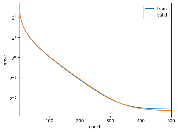
折 1,训练 log rmse: 0.169430, 验证 log rmse: 0.160753
折 2,训练 log rmse: 0.159886, 验证 log rmse: 0.173186
折 3,训练 log rmse: 0.160932, 验证 log rmse: 0.172761
3-折验证: 平均训练log rmse: 0.163416, 平均验证log rmse: 0.168900
保存为 CSV #
不同于上面的 K 折检验, 在实际提交 kaggle 时,要将所有的训练集传入训练
def train_and_pred(train_features, test_features, train_labels, test_data,
                   num_epochs, lr, weight_decay, batch_size):
    net = get_net()
    train_ls, _ = train(net, train_features, train_labels, None, None,
                        num_epochs, lr, weight_decay, batch_size)
    plt.plot(range(1, num_epochs + 1), train_ls, label='train')  # 训练损失
    plt.xlabel('epoch')
    plt.ylabel('rmse')
    plt.xlim([1, num_epochs])
    plt.yscale('log', base=2)  # y 轴使用对数尺度
    plt.legend()
    plt.show()

    print(f'训练log rmse:{float(train_ls[-1]):f}')

    # 将网络应用于测试集。
    preds = net(test_features).detach().numpy() # 将 tensor 不在跟踪梯度,并转为标量
    # 将其重新格式化以导出到 CSV 格式
    test_data['SalePrice'] = pd.Series(preds.reshape(1, -1)[0])
    submission = pd.concat([test_data['Id'], test_data['SalePrice']], axis=1) # 只保留 id 和预测价格
    submission.to_csv('submission.csv', index=False)
num_epochs = 1500
lr = 2
weight_decay = 1e-3
batch_size = 128

train_and_pred(train_features, test_features, train_labels, test_data,
               num_epochs, lr, weight_decay, batch_size)
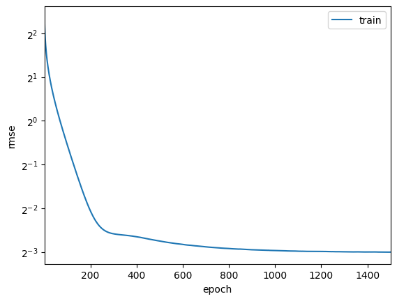
训练log rmse:0.124836
MLP 和多种优化 #
单独一个线性层的成绩并不好
将单独的线性层换成多重感知机
# 测试 cuda
import torch
device = torch.device("cuda" if torch.cuda.is_available() else "cpu")
print(device)
cuda
进行特征工程 #
将 input 进行 transform
# 检查列名
print(train_data.iloc[0, :])
print("-------------")
print(test_data.iloc[0, :])
# 其中 test_data 没有最后的 SalePrice
Id                    1
MSSubClass           60
MSZoning             RL
LotFrontage        65.0
LotArea            8450
                  ...
MoSold                2
YrSold             2008
SaleType             WD
SaleCondition    Normal
SalePrice        208500
Name: 0, Length: 81, dtype: object
-------------
Id                 1461
MSSubClass           20
MSZoning             RH
LotFrontage        80.0
LotArea           11622
                  ...
MiscVal               0
MoSold                6
YrSold             2010
SaleType             WD
SaleCondition    Normal
Name: 0, Length: 80, dtype: object
显然 id 这一列对数据预测没有实际意义
对特征进行整合,并准备进行特征工程
features = pd.concat((train_data.iloc[:, 1:-1], test_data.iloc[:, 1:]))
print(features.shape)
print("--------")
print(features.iloc[0, :])
(2919, 79)
--------
MSSubClass           60
MSZoning             RL
LotFrontage        65.0
LotArea            8450
Street             Pave
                  ...
MiscVal               0
MoSold                2
YrSold             2008
SaleType             WD
SaleCondition    Normal
Name: 0, Length: 79, dtype: object
将数组进行归一化,如公式所示 $$ (x - \mu) / \sigma$$
# numeric_features 是特征中非对象类型(即整数与浮点数)的 index
numeric_features = features.dtypes[features.dtypes != 'object'].index
features[numeric_features] = features[numeric_features].apply(
    lambda x: (x - x.mean()) / (x.std()))
# 在标准化数据之后,所有均值消失。因此我们可以将缺失值设置为 0
features[numeric_features] = features[numeric_features].fillna(0)
在新版本下,get_dummies 会转化为 uint8
但 uint8 不能转化为 numpy,因此要使用 dtype=int
# 接下来处理布尔值。dummy_na 表示是否单独提出 nan
features = pd.get_dummies(features, dummy_na=True, dtype=int)
features.shape
(2919, 330)
进行主成分分析,并划分训练集、测试集
from torch import nn
from sklearn.decomposition import PCA
import torch
n_train = train_data.shape[0]
# 强制将 object 转为 float64
# features = features.astype(str)  # 先将所有列转换为字符串
# features = features.apply(pd.to_numeric, errors='coerce')
pca = PCA(n_components=100)
features_pca = pca.fit_transform(features)
print(features_pca.shape)
train_features = torch.tensor(features[:n_train].values, dtype=torch.float32)
test_features = torch.tensor(features[n_train:].values, dtype=torch.float32)
(2919, 100)
对主成分分析进行可视化,看一下累计贡献图
import seaborn as sns
import matplotlib.pyplot as plt
explained_variance_ratio = np.cumsum(pca.explained_variance_ratio_)

# 图一 累计主成分贡献图
plt.figure(figsize=(10, 6))
plt.plot(range(1, 101), explained_variance_ratio, marker='o', linestyle='--', color='b')
plt.xlabel("Number of Principal Components")
plt.ylabel("Cumulative Explained Variance Ratio")
plt.title("PCA Cumulative Explained Variance")
plt.grid()

plt.axhline(y=0.80, color='r', linestyle='--', label="80% Explained Variance")
plt.axhline(y=0.90, color='g', linestyle='--', label="90% Explained Variance")
plt.legend()
plt.show()

# 图二 具体成果贡献图
explained_variance = pca.explained_variance_ratio_
top_10_components = np.argsort(explained_variance)[-20:][::-1]

loadings = pd.DataFrame(pca.components_, columns=features.columns, index=[f"PC{i+1}" for i in range(100)])

top_10_loadings = loadings.iloc[top_10_components]

top_20_features = top_10_loadings.abs().sum().nlargest(40).index
top_10_loadings = top_10_loadings[top_20_features]

plt.figure(figsize=(14, 8))
sns.heatmap(top_10_loadings, cmap="coolwarm", annot=False, linewidths=0.5)
plt.xlabel("Top 40 Most Important Features")
plt.ylabel("Top 20 Principal Components")
plt.title("Feature Contributions to Top 10 Principal Components")
plt.show()
# 计算均值和标准差
sale_price = np.array(train_data.SalePrice.values, dtype=np.float32).reshape(-1, 1)
mean = sale_price.mean()
std = sale_price.std()

normalized = (sale_price - mean) / std

# 转换为 PyTorch Tensor
train_labels = torch.from_numpy(normalized)
print(train_labels)
tensor([[ 0.3473],
        [ 0.0073],
        [ 0.5362],
        ...,
        [ 1.0776],
        [-0.4885],
        [-0.4208]])
模型搭建 #
下面开始进行线性回归训练,选择 MSE 做 loss。
为了方便对比其他模型,线性回归是一个好的 baseline。
loss = nn.MSELoss()
input_features = features.shape[1] # 其中 shape[1] 是列数,也就是特征数
def get_net():
    net = nn.Sequential(
        nn.Linear(input_features, 256),
        nn.ReLU(),
        nn.Dropout(0.5),
        nn.Linear(256, 64),
        nn.ReLU(),
        nn.Dropout(0.5),
        nn.Linear(64, 1)
    )
    return net
然而,房价的差异在自身房价不同的情况下,不能直接用 abs(target - predict) 直接代表误差
此题官方使用的是 $$ \sqrt {\frac {1}{n} \sum _ {i=1}^ {n} (\log y_ {i}-\log _ {y}i)^ {2} }$$ .
即 均方根对数误差(RMSLE)
而其配合 MSE 就是 均方根对数误差(MSLE)
此外,为保证均方根的合理性,要将 tensor 切割在 (1, inf) 之间
numpy 的 clip() 和 tensor 的 clamp() 作用相同
def log_rmse(net, features, labels, device):
    # 为了在取对数时进一步稳定该值,将小于 1 的值设置为 1
    features, labels = features.to(device), labels.to(device)  # 只添加这一行
    test_labels = (labels.clone() * std) + mean
    clipped_preds = torch.clamp(net(features).clone() * std + mean, 1, float('inf'))
    rmse = torch.sqrt(loss(torch.log(clipped_preds),
                           torch.log(test_labels)))

    return rmse.item()
下面开始训练代码
from torch.utils.data import TensorDataset, DataLoader
from tqdm import tqdm
def train(net, train_features, train_labels, test_features, test_labels,
          num_epochs, learning_rate, weight_decay, batch_size, device):
    net.to(device)

    train_features, train_labels = train_features.to(device), train_labels.to(device)

    if test_features is not None and test_labels is not None:
        test_features, test_labels = test_features.to(device), test_labels.to(device)

    train_ls, test_ls = [], []

    # 用 Dataset 和 DataLoader 进行打包
    dataset = TensorDataset(train_features, train_labels)
    train_iter = DataLoader(dataset, batch_size=batch_size, shuffle=True)

    optimizer = torch.optim.Adam(net.parameters(),
                                 lr=learning_rate,
                                 weight_decay=weight_decay)

    for epoch in tqdm(range(num_epochs), desc="Training"):
        net.train()  # 进入训练模式
        for X, y in train_iter:
            X, y = X.to(device), y.to(device)  # 确保数据在 GPU 上
            optimizer.zero_grad()
            l = loss(net(X), y)  # 计算损失
            l.backward()
            optimizer.step()

        # 记录训练损失
        net.eval()
        train_ls.append(log_rmse(net, train_features, train_labels, device))  # 确保 loss 计算时数据在 GPU 上

        if test_labels is not None:
            test_ls.append(log_rmse(net, test_features, test_labels, device))
    return train_ls, test_ls
K 折交叉检验 #
import matplotlib.pyplot as plt
# 划分 K 折交叉验证数据集
def get_k_fold_data(k, fold_idx, X, y):
    assert k > 1
    fold_size = X.shape[0] // k  # 每折数据大小

    X_valid = X[fold_idx * fold_size: (fold_idx + 1) * fold_size, :]
    y_valid = y[fold_idx * fold_size: (fold_idx + 1) * fold_size]

    # 训练集由剩余 k-1 份数据组成 (即 留一法)
    X_train_parts = []
    y_train_parts = []

    for i in range(k):
        if i == fold_idx:
            continue
        X_part = X[i * fold_size: (i + 1) * fold_size, :]
        y_part = y[i * fold_size: (i + 1) * fold_size]
        X_train_parts.append(X_part)
        y_train_parts.append(y_part)

    # 拼接所有训练集部分
    X_train = torch.cat(X_train_parts, dim=0) # dim = 0 表示按照行合并
    y_train = torch.cat(y_train_parts, dim=0)

    return X_train, y_train, X_valid, y_valid

# 执行 k 折检验
def k_fold(k, X_train, y_train, num_epochs, lr, weight_decay, batch_size, device):
    train_loss_sum, valid_loss_sum = 0, 0

    for fold in range(k): # 进行 K 次留一法
        X_tr, y_tr, X_val, y_val = get_k_fold_data(k, fold, X_train, y_train)

        net = get_net()
        train_ls, valid_ls = train(net, X_tr, y_tr, X_val, y_val,
                                   num_epochs, lr, weight_decay, batch_size, device)

        # 记录 loss_sum (只记录训练每折训练结束的 loss)
        train_loss_sum += train_ls[-1]
        valid_loss_sum += valid_ls[-1]

        # 仅在第一折时绘制损失曲线
        if fold == 0:
            # 画图
            plt.plot(range(1, num_epochs + 1), train_ls, label='train')  # 训练损失
            plt.plot(range(1, num_epochs + 1), valid_ls, label='valid')  # 验证损失

            plt.xlabel('epoch')
            plt.ylabel('rmse')
            plt.xlim([1, num_epochs])
            plt.yscale('log', base=2)  # y 轴使用对数尺度
            plt.legend()
            plt.show()

        print(f'折 {fold + 1},训练 log rmse: {float(train_ls[-1]):.6f}, '
              f'验证 log rmse: {float(valid_ls[-1]):.6f}')

    return train_loss_sum / k, valid_loss_sum / k


num_epochs = 1000
lr = 0.0001
k = 3
weight_decay = 1e-3
batch_size = 512

train_l, valid_l = k_fold(k, train_features, train_labels, num_epochs, lr,
                          weight_decay, batch_size, device)
print(f'{k}-折验证: 平均训练log rmse: {float(train_l):f}, '
      f'平均验证log rmse: {float(valid_l):f}')
Training: 100%|██████████| 1000/1000 [00:11<00:00, 83.82it/s]
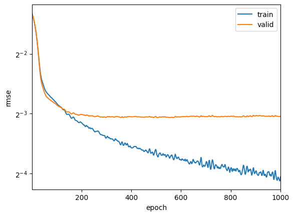
折 1,训练 log rmse: 0.060021, 验证 log rmse: 0.121284


Training: 100%|██████████| 1000/1000 [00:12<00:00, 81.13it/s]


折 2,训练 log rmse: 0.059339, 验证 log rmse: 0.133545


Training: 100%|██████████| 1000/1000 [00:12<00:00, 82.40it/s]

折 3,训练 log rmse: 0.060882, 验证 log rmse: 0.133310
3-折验证: 平均训练log rmse: 0.060081, 平均验证log rmse: 0.129380
保存为 CSV #
不同于上面的 K 折检验, 在实际提交 kaggle 时,要将所有的训练集传入训练
import matplotlib.pyplot as plt
def train_and_pred(train_features, test_features, train_labels, test_data,
                   num_epochs, lr, weight_decay, batch_size):
    net = get_net().to(device)
    train_ls, _ = train(net, train_features, train_labels, None, None,
                        num_epochs, lr, weight_decay, batch_size, device)
    plt.plot(range(1, num_epochs + 1), train_ls, label='train')  # 训练损失
    plt.xlabel('epoch')
    plt.ylabel('rmse')
    plt.xlim([1, num_epochs])
    plt.yscale('log', base=2)  # y 轴使用对数尺度
    plt.legend()
    plt.show()

    print(f'训练log rmse:{float(train_ls[-1]):f}')

    # 将网络应用于测试集。
    preds = net(test_features.to(device)).detach().cpu().numpy() # 将 tensor 不再跟踪梯度,并转为标量
    preds = preds * std + mean
    # 将其重新格式化以导出到 CSV 格式
    test_data['SalePrice'] = pd.Series(preds.reshape(1, -1)[0])
    submission = pd.concat([test_data['Id'], test_data['SalePrice']], axis=1) # 只保留 id 和预测价格
    submission.to_csv('submission.csv', index=False)
num_epochs = 2000
lr = 0.0001
k = 3
weight_decay = 1e-3
batch_size = 512

train_and_pred(train_features, test_features, train_labels, test_data,
               num_epochs, lr, weight_decay, batch_size)
Training: 100%|██████████| 2000/2000 [00:34<00:00, 58.16it/s]
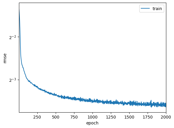
训练log rmse:0.083971
五、结论与讨论 #
1. 线性回归:简单但有效 #
最开始,我选择了最基础的线性回归模型,实际上 PyTorch 里 nn.Linear() 就能轻松实现。虽然简单,但只要数据预处理得当,比如归一化、数据类型转换、独热编码等,线性回归的效果其实也不错。
在这个过程中,我发现 K 折交叉验证 是个非常重要的工具,它让我能更客观地评估模型的泛化能力,避免单次训练结果的偶然性。此外,损失函数的选择 也很关键,这里 MSELoss()(均方误差)效果最好,而 RMSE(均方根误差)更适合作为最终评估指标。
小结:线性回归虽然简单,但如果数据处理得当,表现并不差,甚至可以作为一个可靠的基线模型。
2. MLP:神经网络并不总是更好 #
接下来,我尝试把线性模型升级成 MLP(多层感知机),希望它能学到更复杂的特征。然而,模型刚训练出来就发现了一个大问题:严重的过拟合。
为什么会这样?主要有两个原因:
- MLP 结构过于复杂,参数太多,导致模型学到了很多无关的噪声数据。
- 损失函数 MSE 在不同房价区间的影响不同,高价房的误差会被放大。
为了解决这些问题,我做了几项调整:
- 加入 Dropout(0.5)和 L2 正则化,减少过拟合
- 对标签归一化,让 MSE 在不同房价区间的影响更均衡
- 使用 PCA(主成分分析)降维,减少无关特征
结果确实有提升,但神经网络并不是万能的,如果数据特征没选好,模型再复杂也没用。
小结:神经网络并不总是比线性回归好,尤其是数据量不大时,复杂模型反而容易过拟合。
3. 特征工程才是关键 #
在调整 MLP 的过程中,我逐渐意识到:模型的选择往往没那么重要,真正决定表现的其实是数据本身。
后来,我参考了一些别人的思路,尝试从特征工程入手,比如:
- 针对房价预测的特性,设计更合适的特征
- 结合已有的高分测试集,调整特征组合方式
调整之后,模型的表现确实更好了,但这个过程让我有些思考: 这些优化是否真的有普遍适用性?如果换个数据集,效果还会这么好吗?
小结:模型的复杂度并不是提升效果的关键,如何处理数据、如何提取有用特征,才是真正决定模型表现的核心。
4. 我的感悟 #
简单模型+好数据 > 复杂模型+普通数据,线性回归如果数据处理得当,效果不会比 MLP 差太多。